最小二乘法

• 日用而不知
• 最小二乘法
• 推广
• 最小二乘法的矩阵法解法
• 最小二乘法与正态分布
• 案例python实现
• 正则化
• 参考

日用而不知

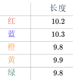
来看一个生活中的例子。比如说，有五把尺子：

用它们来分别测量一线段的长度，得到的数值分别为（颜色指不同的尺子）：

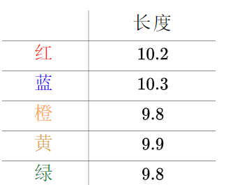
之所以出现不同的值可能因为：

• 不同厂家的尺子的生产精度不同
• 尺子材质不同，热胀冷缩不一样
• 测量的时候心情起伏不定
• ……

总之就是有误差，这种情况下，一般取平均值来作为线段的长度：

总之就是有误差，这种情况下，一般取平均值来作为线段的长度：

日常中就是这么使用的。可是作为很事’er的数学爱好者，自然要想下：

• 这样做有道理吗？
• 用调和平均数行不行？
• 用中位数行不行？
• 用几何平均数行不行？

最小二乘法

换一种思路来思考刚才的问题。

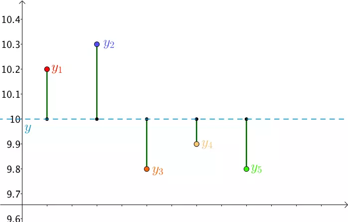
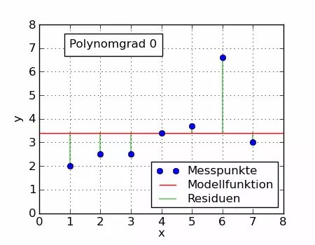
首先，把测试得到的值画在笛卡尔坐标系中，分别记作 $y_i$

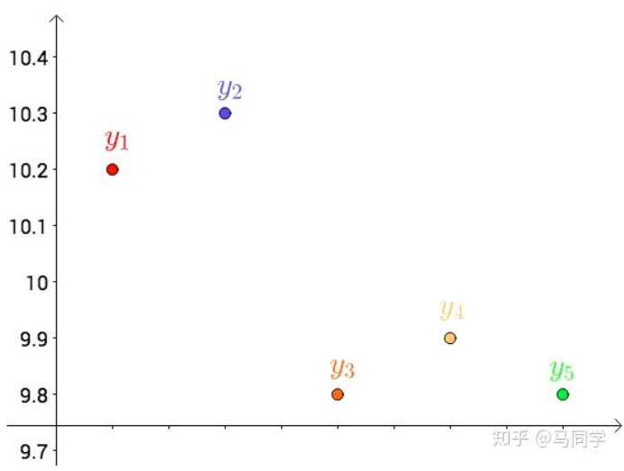
其次，把要猜测的线段长度的真实值用平行于横轴的直线来表示（因为是猜测的，所以用虚线来画），记作 $y$

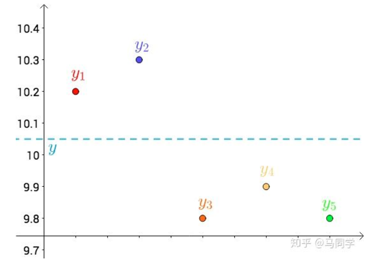
每个点都向 $y$ 做垂线，垂线的长度就是 $|y-y_{i}|$，也可以理解为测量值和真实值之间的误差：

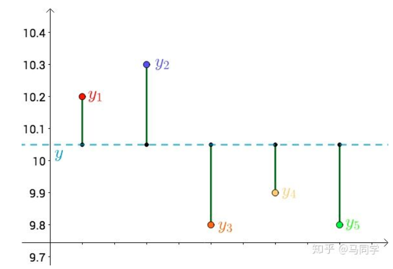
因为误差是长度，还要取绝对值，计算起来麻烦，就干脆用平方来代表误差：

误差的平方和就是（\(\epsilon\) 代表误差）：

因为 $y$ 是猜测的，所以可以不断变换：

自然，误差的平方和\(S_{\epsilon^{2}}\) 在不断变化的。

法国数学家，阿德里安-马里·勒让德, 提出让总的误差的平方最小的 $y$ 就是真值，这是基于，如果误差是随机的，应该围绕真值上下波动

勒让德的想法变成代数式就是：

这是一个二次函数，对其求导，导数为0的时候取得最小值：

进而：

正好是算术平均数。

原来算术平均数可以让误差最小啊，这下看来选用它显得讲道理了。

以下这种方法：

就是最小二乘法，所谓“二乘”就是平方的意思，台湾直接翻译为最小平方法。

推广

算术平均数只是最小二乘法的特例，适用范围比较狭窄。而最小二乘法用途就广泛。

比如温度与冰淇淋的销量：

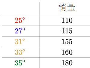
看上去像是某种线性关系：

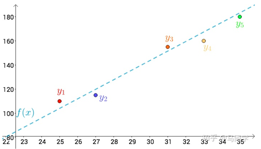
可以假设这种线性关系为： \(\begin{equation}f(x)=a x+b\end{equation}\) 通过最小二乘法的思想：

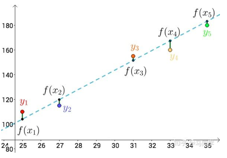
上图的 $i, x, y$ 分别为：

总误差的平方为：

不同的 $a, b$ 会导致不同的 \(S_{\epsilon^{2}}\)，根据多元微积分的知识，当：

这个时候 \(S_{\epsilon^{2}}\) 取最小值。

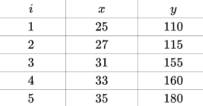
对于 $a,b$ 而言，上述方程组为线性方程组，用之前的数据解出来：

也就是这根直线：

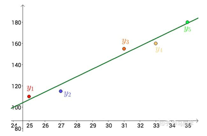
其实，还可以假设：

在这个假设下，可以根据最小二乘法，算出 $a,b,c$ ，得到下面这根红色的二次曲线：

同一组数据，选择不同的 $f(x)$ ，通过最小二乘法可以得到不一样的拟合曲线

不同的数据，更可以选择不同的 $f(x)$ ，通过最小二乘法可以得到不一样的拟合曲线：

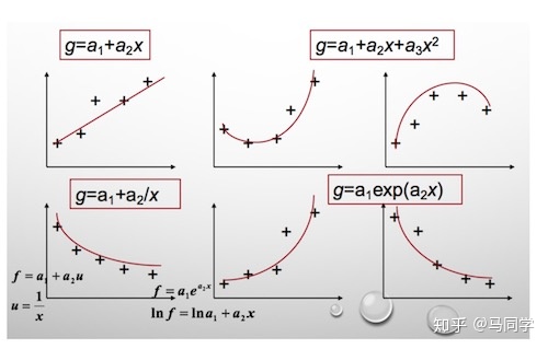
$f(x)$ 也不能选择任意的函数，还是有一些讲究的.

最小二乘法的矩阵法解法

比如我们有 个只有一个特征的样本 \(\left(x_{i}, y_{i}\right)(i=1,2,3 \ldots, m)\)

样本采用一般的 为 次的多项式拟合，

\(h_{\theta}(x)=\theta_{0}+\theta_{1} x+\theta_{2} x^{2}+\ldots \theta_{n} x^{n}, \theta\left(\theta_{0}, \theta_{1}, \theta_{2}, \ldots, \theta_{n}\right)\) 为参数

最小二乘法就是要找到一组 \(\theta\left(\theta_{0}, \theta_{1}, \theta_{2}, \ldots, \theta_{n}\right)\) 使得 \(\sum_{i=1}^{n}\left(h_{\theta}\left(x_{i}\right)-y_{i}\right)^{2}\) (残差平方和) 最小，即，求 \(\min \sum_{i=1}^{n}\left(h_{\theta}\left(x_{i}\right)-y_{i}\right)^{2}\)

最小二乘法的代数法解法就是对 求偏导数，令偏导数为 0，再解方程组，得到 。矩阵法比代数法要简洁，下面主要讲解下矩阵法解法，这里用多元线性回归例子来描：

假设函数

的矩阵表达方式为：

其中， 假设函数 为 的向量, 为 的向量，里面有 个代数法的模型参数。 为 维的矩阵。 代表样本的个数， 代表样本的特征数。

损失函数定义为:

其中 是样本的输出向量，维度为 。 在这主要是为了求导后系数为1，方便计算。

根据最小二乘法的原理，我们要对这个损失函数对 向量求导取0。结果如下式：

对上述求导等式整理后可得：

最小二乘法与正态分布

我们对勒让德的猜测，即最小二乘法，仍然抱有怀疑，万一这个猜测是错误的怎么办？

数学王子高斯（1777－1855）也像我们一样心存怀疑。

高斯换了一个思考框架，通过概率统计那一套来思考。

让我们回到最初测量线段长度的问题。高斯想，通过测量得到了这些值：

每次的测量值 $x_i$ 都和线段长度的真值 $x$ 之间存在一个误差： \(\begin{equation}\epsilon_{i}=x-x_{i}\end{equation}\) 这些误差最终会形成一个概率分布，只是现在不知道误差的概率分布是什么。假设概率密度函数为： \(\begin{equation}p(\epsilon)\end{equation}\)

再假设一个联合概率，这样方便把所有的测量数据利用起来：

把 $x$ 作为变量的时候，上面就是似然函数了

$L(x)$的图像可能是这样的（随便画的）：

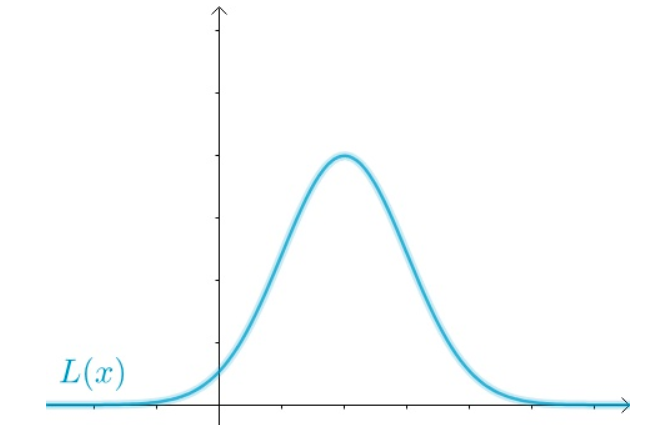
根据极大似然估计的思想，联合概率最大的最应该出现（既然都出现了，而我又不是“天选之子”，那么自然不会是发生了小概率事件）, 也就是应该取到下面这点：

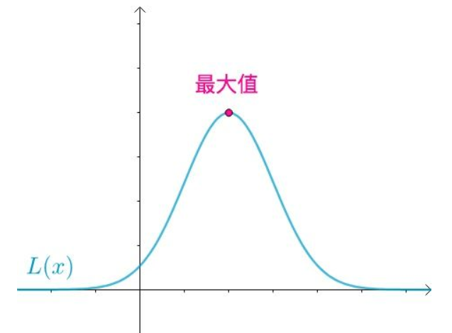
当下面这个式子成立时，取得最大值：

然后高斯想，最小二乘法给出的答案是：

如果最小二乘法是对的，那么 $x=\bar{x}$ 时应该取得最大值，即：

好，现在可以来解这个微分方程了。最终得到：

这是什么？这就是正态分布啊。

并且这还是一个充要条件：

也就是说，如果误差的分布是正态分布，那么最小二乘法得到的就是最有可能的值。

那么误差的分布是正态分布吗？

如果误差是由于随机的、无数的、独立的、多个因素造成的，比如之前提到的：

• 不同厂家的尺子的生产精度不同
• 尺子材质不同，热胀冷缩不一样
• 测量的时候心情起伏不定
• ………

虽然勒让德提出了最小二乘法（高斯说他最早提出最小二乘法，只是没有发表），但是高斯的努力，才真正奠定了最小二乘法的重要地位。

案例python实现

目标函数

导入库函数

import numpy as np
import pandas as pd
from scipy.optimize import leastsq
import matplotlib.pyplot as plt

%matplotlib inline
%load_ext lab_black

定义目标函数，多项式函数，残差函数

# 目标函数
def real_func(x):
    return np.sin(2 * np.pi * x)


# 多项式
def fit_func(p, x):
    f = np.poly1d(p)
    return f(x)


# 残差
def residuals_func(p, x, y):
    ret = fit_func(p, x) - y
    return ret

添加随机误差

# 十个点
x = np.linspace(0,1,10)
x_points = np.linspace(0,1,1000)

# 加上正态分布噪音的目标函数的值
y_ = real_func(x)
y = [np.random.normal(0,0.1)+y1 for y1 in y_]

拟合多项式并可视化

def fitting(M=0):
    """
    M :  多项式的次数
    """
    # 随机初始化多项式的参数
    p_init = np.random.rand(M + 1)

    # 最小二乘法
    p_lsq = leastsq(residuals_func, p_init, args=(x, y))
    print(f"Fitting Parameters{p_init[0]}")

    # 可视化
    plt.plot(x_points, real_func(x_points), label="real")
    plt.plot(x_points, fit_func(p_lsq[0], x_points), label="fitted curve")
    plt.plot(x, y, "bo", label="noise")
    plt.legend()
    plt.savefig(f"{M}.png", dpi=300)
    return p_lsq

• 0 次拟合

  p_lsq_0 = fitting(M=0)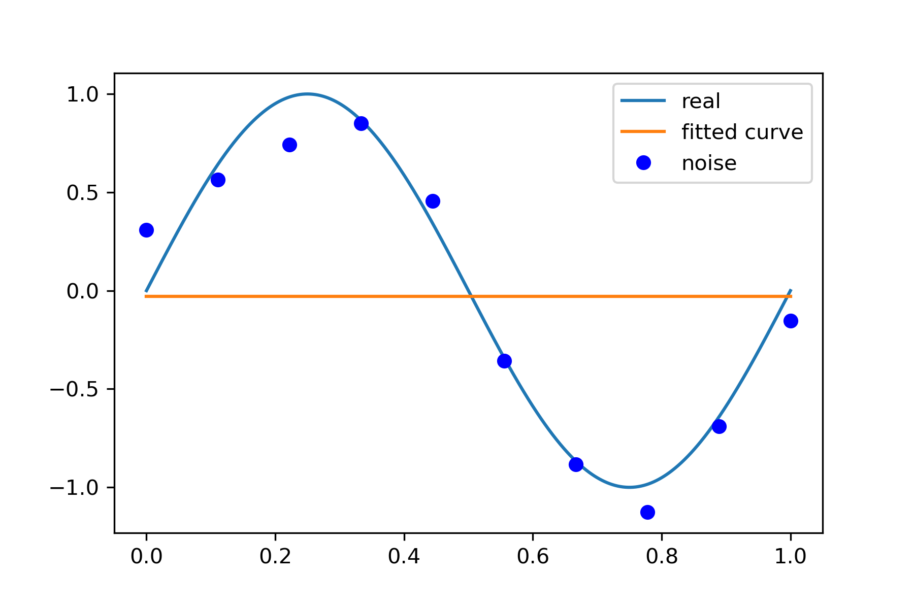
  

  

• 1 次拟合

  # M=1
  p_lsq_1 = fitting(M=1)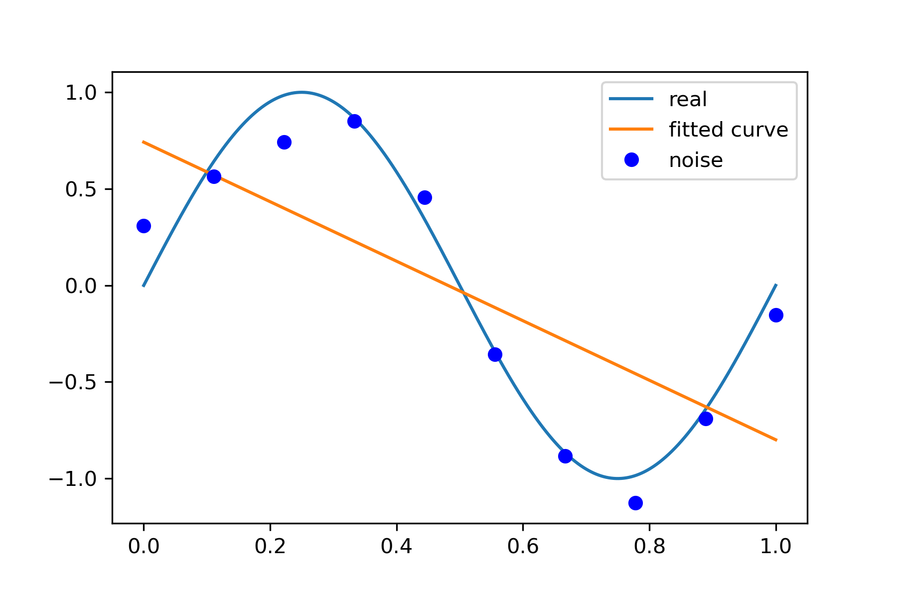
  

  

• 3 次拟合

  # M=3
  p_lsq_3 = fitting(M=3)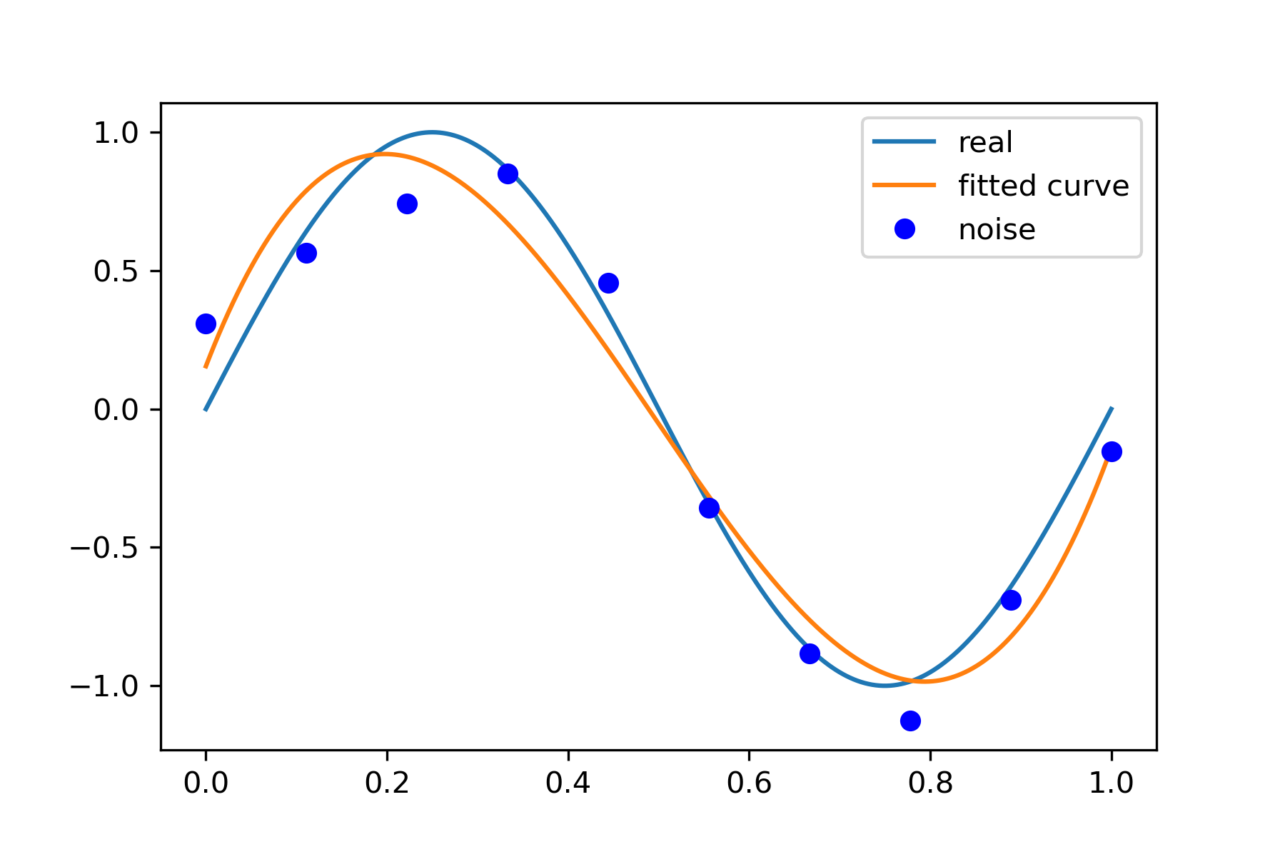
  

  

• 9 次拟合

  # M=9
  p_lsq_9 = fitting(M=9)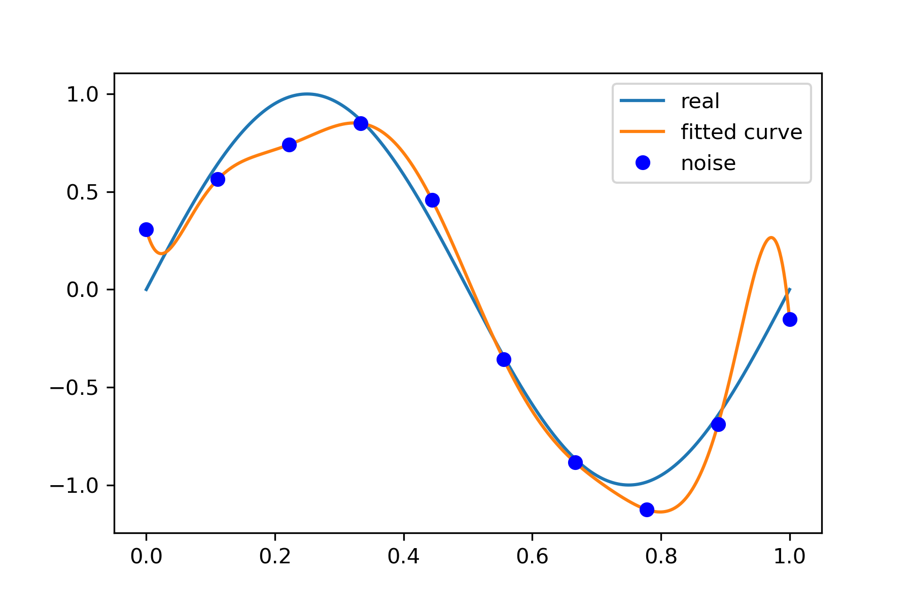
  

  

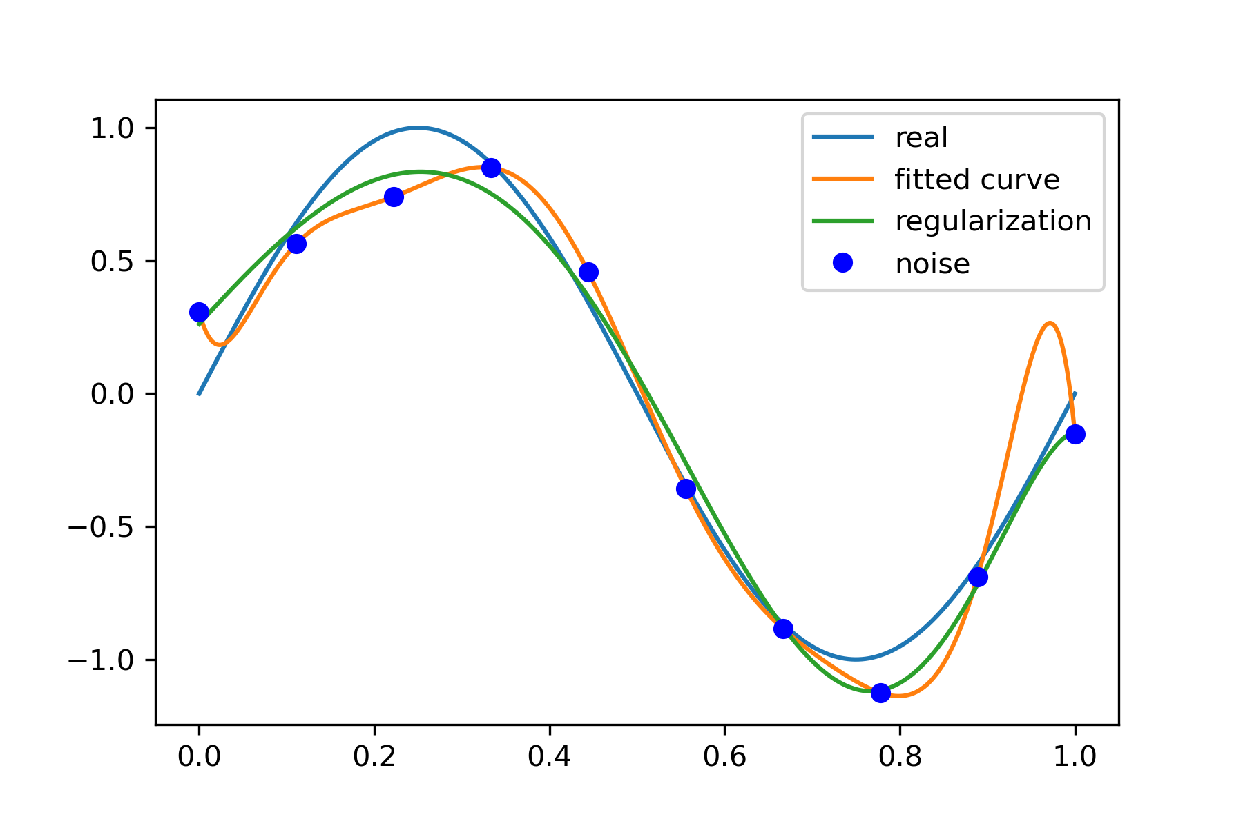
当M=9时，多项式曲线通过了每个数据点，但是造成了过拟合

正则化

结果显示过拟合， 引入正则化项(regularizer)，降低过拟合

回归问题中，损失函数是平方损失，正则化可以是参数向量的L2范数,也可以是L1范数。

L1: regularization*abs(p)

L2: 0.5 * regularization * np.square(p)

regularization = 0.0001


def residuals_func_regularization(p, x, y):
    ret = fit_func(p, x) - y
    ret = np.append(ret, np.sqrt(0.5 * regularization * np.square(p)))
    return ret

# 最小二乘法,加正则化项
p_init = np.random.rand(9 + 1)
p_lsq_regularization = leastsq(residuals_func_regularization, p_init, args=(x, y))

plt.plot(x_points, real_func(x_points), label="real")
plt.plot(x_points, fit_func(p_lsq_9[0], x_points), label="fitted curve")
plt.plot(x_points, fit_func(p_lsq_regularization[0], x_points), label="regularization")
plt.plot(x, y, "bo", label="noise")
plt.legend()

参考

• 最小二乘法的本质是什么？
• 最小二乘法（least sqaure method）